import matplotlib.pyplot as plt
import numpy as np

t = np.arange(0.0, 5.0, 0.01)
s = np.cos(2 * np.pi * t)

line = plt.plot(t, s, lw=2)
plt.show()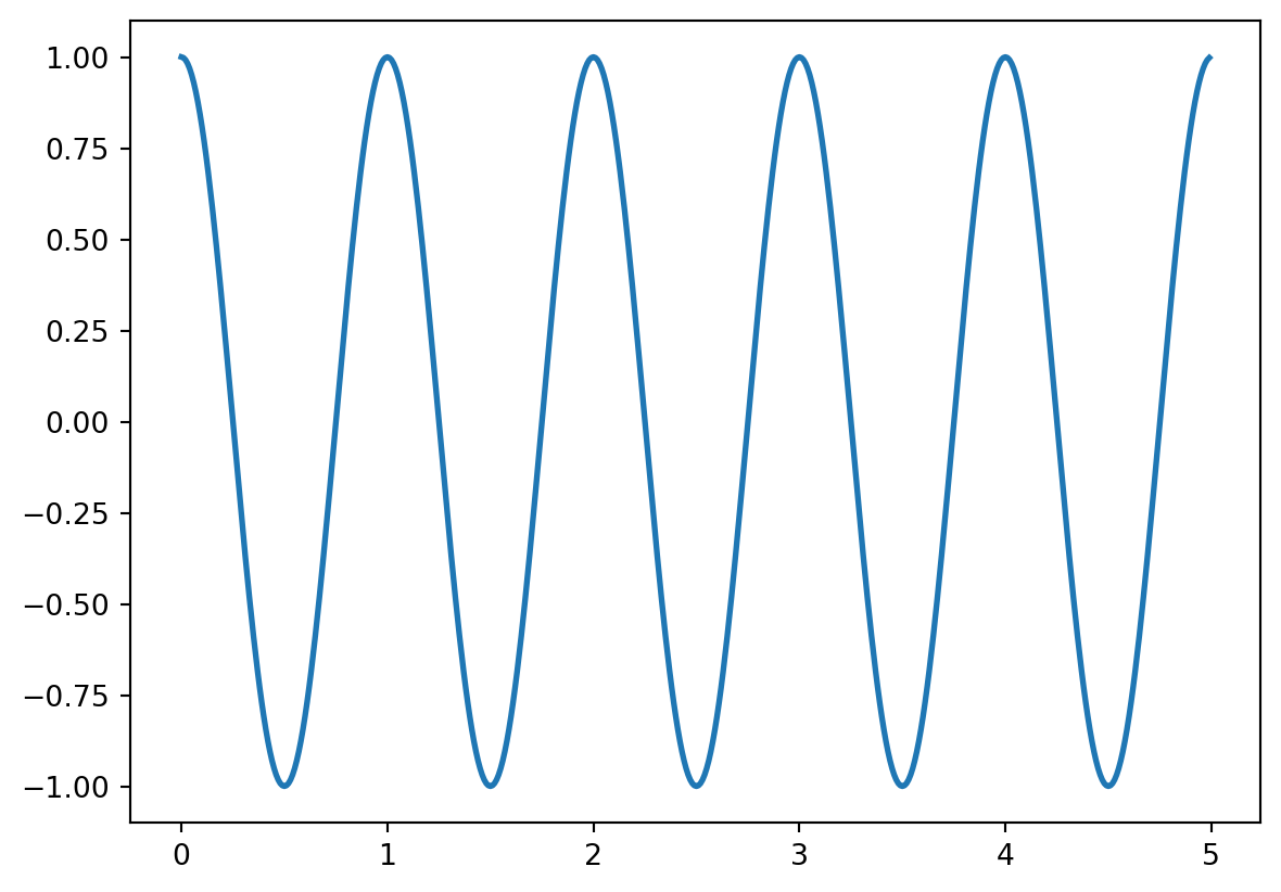
import matplotlib.pyplot as plt
import numpy as np
t = np.arange(0.0, 5.0, 0.01)
s = np.cos(2 * np.pi * t)
line = plt.plot(t, s, lw=2)
plt.show()
Lorem ipsum
Pangeo Forge provides efficient, cloud-optimized access to large datasets.
Lets use xarray to access Pangeo Forge’s NOAA Coastwatch Geo-Polar SST dataset. This dataset was added to Pangeo Forge via a recipe maintained in a pangeo-forge feedstock repository from data hosted at NOAA (Coastwatch 2023).
import xarray as xr

store = 'https://ncsa.osn.xsede.org/Pangeo/pangeo-forge/noaa-coastwatch-geopolar-sst-feedstock/noaa-coastwatch-geopolar-sst.zarr'
ds = xr.open_dataset(store, engine='zarr', chunks={})Lets select a slice (2012-09-16, the date of the record sea ice minimum per the Sea Ice index) out of the sea surface temperature (sst) variable.
sst_20120916 = ds.analysed_sst.sel(time='20120916', method='nearest')Now lets take a look at the data!
import matplotlib.pyplot as plt

img = sst_20120916.plot.imshow()
plt.show()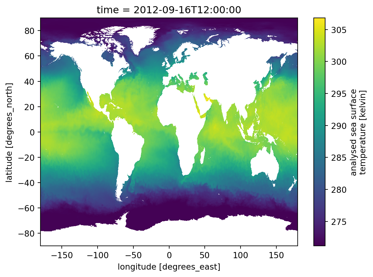
Remember how we already plotted some data with matplotlib earlier? See Figure 1!